From Autoencoders to VAE: Smooth Latent Spaces

Jani Isohanni

31 Mar 2026 • 11 min read

In the previous article we noticed that with autoencoders the learned latent space was very sparse. The locations (points) in latent space that can produce any meaningful images are few and far between. When building generative models this is a problem. We wouldn't want a model that produces meaningful output only with 0.1% of inputs, or even less.

Variational autoencoders, VAEs, solve this issue.

At a high level VAE construction is again rather simple, but to understand why it works, we need to cover the background theory quite a bit.

VAE Architecture

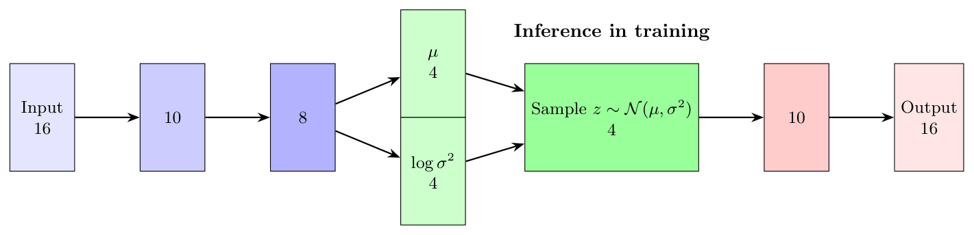
In VAE we introduce stochastic step to the network. In the previous article we had the clear 16 -> 10 -> 4 -> 10 -> 16 layered structure where encoder and decoder are of the same size and latent space is of dimension 4.

In VAE we take the latent space structure into account and instead of constructing the latent representation from input deterministically, we assume \(z\) follows a prior normal distribution and make the encoder compute the mean and variance of that space.

VAE where z is sampled. The figure is from training phase.

The idea sounds simple, and at core it is, but the sampling step causes some headache in backpropagation, because it is not a deterministic step let alone differentiable. Also, it is not that clear what and especially why introducing this step helps.

To make matters even worse, we step away from the convenience of training a model and then using it as-is for inference. In VAE, the forward pass during training differs from the inference phase.

Our journey is towards generative models hence we put effort to understand the latent space construction and decoder.

VAE The Theory

We have training data and the core assumption is that the dataset has meaningful structure to learn. Having training data of \(256\times 256\) images with white noise within wouldn't make much sense, would it? In neural network theory we package this "something to learn from" as a probability density function \(p\).

When we write \(p(x)\), this means that \(x\) is an object in the space of all input objects like RGB images of size \(256\times 256\), and \(p(x)\) states the probability that \(x\) belongs to the subset of all images that we want the system to learn. Usually we don't know what \(p(x)\) is (if we would, there wouldn't be much need to try to learn it in the first place) and we treat the function \(p\) as... well, just a function with not that much extra assumptions. But what we do have is samples from \(p(x)\), i.e. our training data.

Our neural network now tries to learn \(p\) and we model this approximation with \( p_\theta(x)\) where \(\theta\) is decoder weights (and bias). With this notation our goal is to locate \(\theta\) that would make \(p_\theta(x)\) as close to \(p(x)\) as possible.

Before stepping any further, there are some standard notation we need to define. With \(p_\theta\) we refer to decoder and with \(q_\varphi\) to encoder. In VAE we need to conceptually separate the networks. Here encoder extracts the features and we want to control it in a way separately from decoder.

That said.. consider the latent space. We assume that there is some lower dimensional space that can encapsulate the characteristics of \(p(x)\) in latent space vector \(z\) in a way that would allow us to reconstruct \(x\) from \(z\). This means that we make an assumption that there exists distribution \(p_\theta(x,z)\) where \(x\) is the learnable and \(z\) is the latent representation of it.

This assumption with Bayesian rules gives us

\[p_{\theta}(x,z)=p_{\theta}(x\mid z)p(z).\]

Here \(p(z)\) does not depend on \(\theta\) by choice. We want to keep \(p(z)\) fixed because if we would let it to depend on \(\theta\), it would provide too much freedom for the network and that would lead us to sparse latent space with other computational problems. We'll return to this soon.

Continuing with Bayes we get

\[p_{\theta}(x) = \int p_{\theta}(x,z)\,dz = \int p_{\theta}(x\mid z)p(z)\,dz.\]

Here the integral is intractable for the very problem we are trying to solve - the latent space is too sparse to work with. We would end up with zero almost everywhere. And this observation leads us to the very good question: in that case, shouldn't we make the latent space more compact by cutting dimensions, which would lead to less sparse space to work with?

Well, perhaps, but there is an inherent problem within. Should we cut the dimension, we would cut the resolution as well. We don't know upfront where the interesting data actually lives in. For example:

The data can reside in nonlinear subspace (and usually does)
The subspace is not easily parametrizable
The data can reside in a curved and complex manifold

If we consider the example in the previous article or autoencoders, we located ten clear clusters within the latent space because we had very simple data. But when we target a system that can really generate say images from text, we need to have resolution. A lot of resolution, because otherwise it would be very hard to have a system that could separate concepts, which in turn would lead to a system that generates similar or equal output even with varying inputs. The output would be "narrow". Not too compelling scenario.

Clear? Good, lets proceed to encoder.

Again, we have the assumption about the distributions \(p(x)\) and \(p(x,z)\). Encoder's function is to extract the features of the input in a best possible way. We model encoder with \(q_{\varphi}(z\mid x)\) which should by definition approximate \(p(z\mid x)\). We can think \(q_{\varphi}(z\mid x)\) as a posterior distribution that approximates \(p(z\mid x)\).

Now, again with Bayes, we get

\[ p(z\mid x)=\frac{p_{\theta}(x\mid z)p(z)}{p_{\theta}(x)}\]

And the denominator is intractable as noted already. We can solve this by a simple assumption, namely let

\[q_{\varphi}(z\mid x)\sim\mathcal{N}(z\mid\mu_{\varphi(x)}, \sigma^2_{\varphi(x)}).\]

This is the sampling phase in Figure 1. The encoder returns vectors \(\mu\) and \(\log(\sigma^2)\) and we use them to sample \(z\) (in a way).

What we have now is an encoder that returns mean and logarithm of variance. We use them to sample \(z\) to feed to the decoder. Here one must be careful, the actual sampling is usually only done during training. In inference one often sets

\[z = \mu\]

to get deterministic results and ditch the variance.

In high level the decoder is trained to produce \(x\) from \(z\) in such a way that \(p_\theta(x\mid z)\) is maximized. And because the latent space is almost empty, we need to teach encoder to produce such parameters that would fill up the latent space. Or in other words, we teach the encoder to produce distributions that overlap and cover the latent space densely.

What we have is a kind of intermediate layer where the encoder produces the parameters of a normal distribution, based on which samples are generated, from which the decoder attempts to reconstruct \(x\) such that \(p(x)\) is as large as possible. This intermediate layer is clearly not differentiable, so backpropagation cannot work on it even in theory; we have a non-deterministic and moreover non-invertible operation in the middle of the network.

Let's first examine what we are optimizing. The network's success is directly measured by \(p_{\theta}(x)\), so we seek \(\theta\) that maximizes \(p_{\theta}(x)\). For practical reasons (mostly numerical stability), we optimize \(\log⁡(p_{\theta}(x))\) and obtain:

\[\log(p_{\theta}(x))=\log(\int p_{\theta}(x,z)\,dz)=\]

\[\log(\int p_\theta(x,z)\cdot\frac{q_{\varphi}(z\mid x)}{q_{\varphi}(z\mid x)}\, dz)\]

\[=\log( \mathbb{E}_{z\sim q_{\varphi}(z\mid x)}[\frac{p_{\theta}(x,z)}{q_{\varphi} (z\mid x)} ])\]

Use Jensen inequality.

\[\geq \mathbb{E}_{z\sim q_{\varphi}(z\mid x)}[\log(p_{\theta}(x,z)/q_{\varphi}(z\mid x))]\]

\[=\mathbb{E}_{z\sim q_{\varphi}(z\mid x)}[\log(p_{\theta}(x,z))-\log(q_{\varphi}(z\mid x))]\]

This simplifies to the form:

\[ L(\theta, \varphi;x)=\mathbb{E}_{z \sim q_{\varphi}(z\mid x)}[\log(p_{\theta}(x\mid z))] - KL(q_{\varphi}(z\mid x)\|p(z))\]

The next concern is the computation of KL-divergence. But that's why we chose the normal distribution as the prior; it provides a closed form for the divergence. That is, for \(KL(q_{\varphi}(z\mid x)\|p(z))\) where

\[q_{\varphi}(z\mid x) = \mathcal{N}(\mu,\sigma^2)\]

and \(p(z) = \mathcal{N}(0,I)\), we get:
\[KL(\mathcal{N}(\mu,\sigma^2)\|\mathcal{N}(0,I))=0.5*\sum_j [\mu_j^2 + \sigma_j^2 - \log(\sigma_j^2) - 1].\]

Note that \(p(z)\) is chosen as \(\mathcal{N}(0,I)\) and it is constant throughout training. The KL term plays a crucial balancing role here. Without it, the model could minimize reconstruction error by either making \(\sigma\to 0\) (deterministic encoding) or by ignoring \(z\) entirely and learning to generate \(x\) directly from the prior \(p(z)\). This problem is known as posterior collapse. In posterior collapse, the encoder becomes useless as the decoder learns to generate data independently of the input.

The KL penalty prevents this by penalizing the encoder's distribution \(q_{\varphi}(z\mid x)\) from drifting too far from the prior \(p(z)=\mathcal{N}(0,I)\). This keeps the latent codes centered near the origin while maintaining reasonable variance, ensuring that the latent space remains structured and usable for generation.

The first term, on the other hand, is directly the reconstruction error. We'll return to that.

But now we still have the aforementioned non-deterministic sampling in training. This we can overcome through so-called reparameterization. We simply assume that

\[ z = \mu + \sigma\cdot\epsilon\]

where \(\epsilon\) is a random variable from distribution \(\mathcal{N}(0,I)\). This construction enables backpropagation because now \(z\) is computed directly from the weights produced by the encoder, but it simultaneously preserves the stochastic nature of the network through \(\epsilon\).

Mathematically, \(\epsilon\) is "harmless" because during training it is sampled repeatedly from distribution \(\mathcal{N}(0,I)\), hence the mean of samples converges to zero, i.e., it doesn't shift the distribution anywhere. At the same time, \(I\) ensures that the randomness stays in the same form as we assume of the prior. Technically, we thus have a different computation method in the inference phase than what backpropagation sees.

Finally, the definition of reconstruction error remains. This now depends on what kind of distribution we assume \(p_{\theta}(x\mid z)\) to follow. Often the assumption is made that it is a normal distribution, which yields

\[p_{\theta}(x\mid z)\sim\mathcal{N}(x\mid\mu _{\theta(z)},\sigma^2)\]

and we get the error term

\[\log(p_{\theta}(x\mid z)) = \frac{-1}{2\sigma^2}\|x-\mu_{\theta(z)}\|^2 + C\]

where \( C \) is a constant. In this case the error term is proportional to MSE.

But, if instead we assume Bernoulli-distribution

\[p_{\theta}(x\mid z)\sim\prod_i Bernoulli(x_i \mid p_i(z))\]

then decoder produces probability per pixel. Given that we are working with gray scale images that are already scaled to the range \([0,1]\), this is tempting option. In this case the error term would be

\[\log(p_{\theta}(x\mid z)) = \sum_i [x_i\log(p_i)+(1-x_i)\log(1-p_i)]\]

which is binary cross entropy.

VAE the Practise

Reminder, full code is in my GitHub under deep_learning/vae.

Model And Training

We can define the model with PyTorch.

class VAE(nn.Module):
    def __init__(self, latent_dim=2):
        super().__init__()
        # Encoder
        self.fc1 = nn.Linear(784, 400)
        self.fc_mu = nn.Linear(400, latent_dim)
        self.fc_logvar = nn.Linear(400, latent_dim)
        
        # Decoder
        self.fc3 = nn.Linear(latent_dim, 400)
        self.fc4 = nn.Linear(400, 784)
    
    def encode(self, x):
        h = F.relu(self.fc1(x))
        return self.fc_mu(h), self.fc_logvar(h)
    
    def reparameterize(self, mu, logvar):
        std = torch.exp(0.5 * logvar)
        eps = torch.randn_like(std)
        return mu + eps * std
    
    def decode(self, z):
        h = F.relu(self.fc3(z))
        return torch.sigmoid(self.fc4(h))
    
    def forward(self, x):
        mu, logvar = self.encode(x.view(-1, 784))
        z = self.reparameterize(mu, logvar)
        return self.decode(z), mu, logvar
        ```

There are some parts we notice. First, forward return \(\mu\) and \(\log(\sigma^2)\) which we need to be able to calculate KL-term in the loss. This should be clear. More interesting part is the reparameterize-method.

In the theory part, we insisted \(z\) to be sampled from \(\mathcal{N}(\mu,\sigma^2)\) and talked about the reparameterization trick to allow backpropagation. Here we can see how we use \(\epsilon\) to "emulate" sampling from \(\mathcal{N}(\mu,\sigma^2)\). This means we do not sample from \(\mathcal{N}(\mu,\sigma^2)\) directly, but instead use the mean and variance as constants-of-the-moment and \(\epsilon\) is our stochastic variable.

Embedding the \(\epsilon\) to the code this way makes the network technically differentiable and hence trainable with backpropagation.

Now, the loss-function. Here we will use so called \(\beta\)-VAE where the KL-divergence is weighted with \(\beta\). The motivation is to have a parametrization that forces the model to put more effort in making the latent space "more smooth" but the cost is that decoding quality usually degrades when we increase \(\beta\). I would encourage we to try different values for \(\beta\) to get a feeling how it works. Usually we get good results with \(\beta\in[1,10]\) but there is no theoretical limit.

Notice that we minimize the ELBO hence the change of signs.

def loss_function(recon_x, x, mu, logvar):
    # Reconstruction loss (BCE)
    BCE = F.binary_cross_entropy(recon_x, x.view(-1, 784), reduction='sum')
    
    # KL divergence
    KLD = -0.5 * torch.sum(1 + logvar - mu.pow(2) - logvar.exp())
    
    return BCE + beta * KLD
    ```

The hyperparameters in our demonstration are

latent_dim = 4 
batch_size = 128
epochs = 15
learning_rate = 1e-3
beta = 1.0

And we are ready to train.

model = VAE(latent_dim=latent_dim)
optimizer = torch.optim.Adam(model.parameters(), lr=learning_rate)

model.train()
for epoch in range(epochs):
    train_loss = 0
    for batch_idx, (data, _) in enumerate(train_loader):
        optimizer.zero_grad()
        recon_batch, mu, logvar = model(data)
        loss = loss_function(recon_batch, data, mu, logvar)
        loss.backward()
        train_loss += loss.item()
        optimizer.step()
        ```

Results

Let us first visualize the latent space structure mapped to 2D.

model.eval()
with torch.no_grad():
    z_list, labels_list = [], []
    for data, labels in train_loader:
        mu, _ = model.encode(data.view(-1, 784))
        z_list.append(mu)
        labels_list.append(labels)
    
    z = torch.cat(z_list).numpy()
    labels = torch.cat(labels_list).numpy()
    
    plt.figure(figsize=(10, 8))
    reducer = umap.UMAP(random_state=42)
    z_2d = reducer.fit_transform(z)
    ```

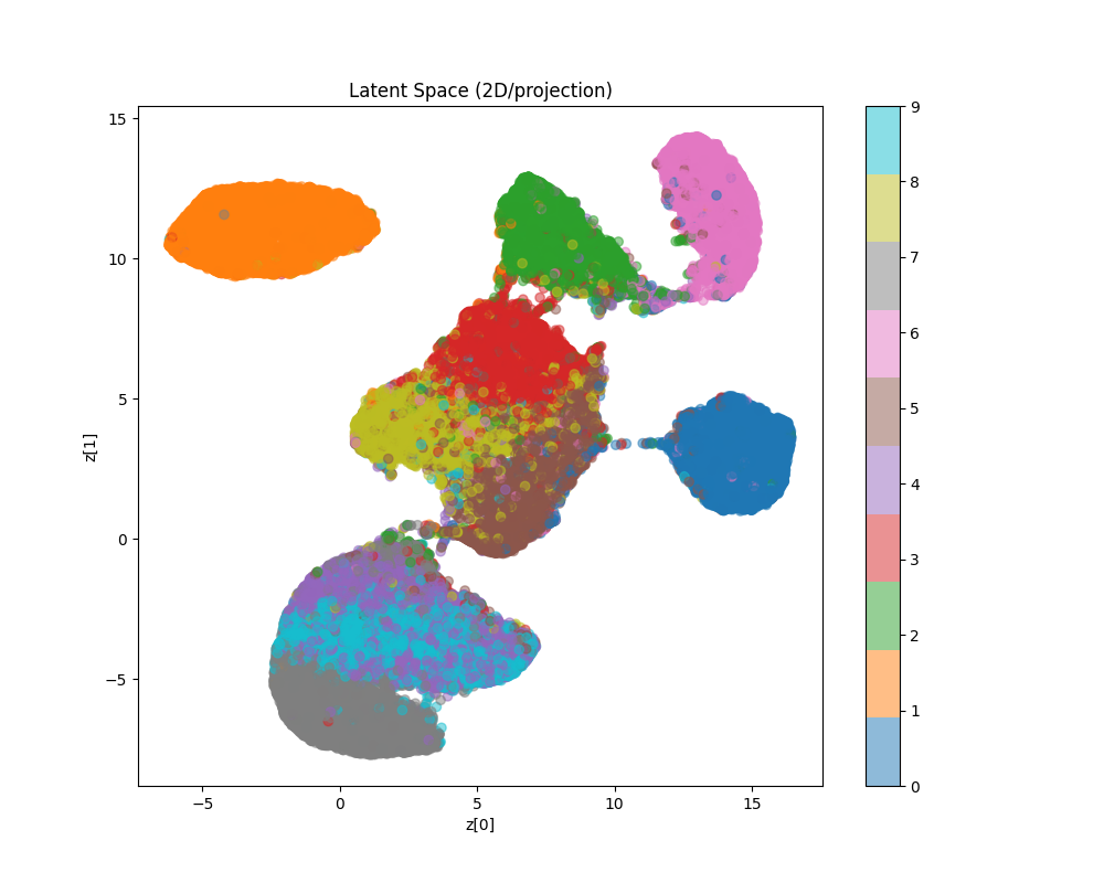
As we can see from the image, the latent space is more continuous compared to what we got from autoencoder alone.

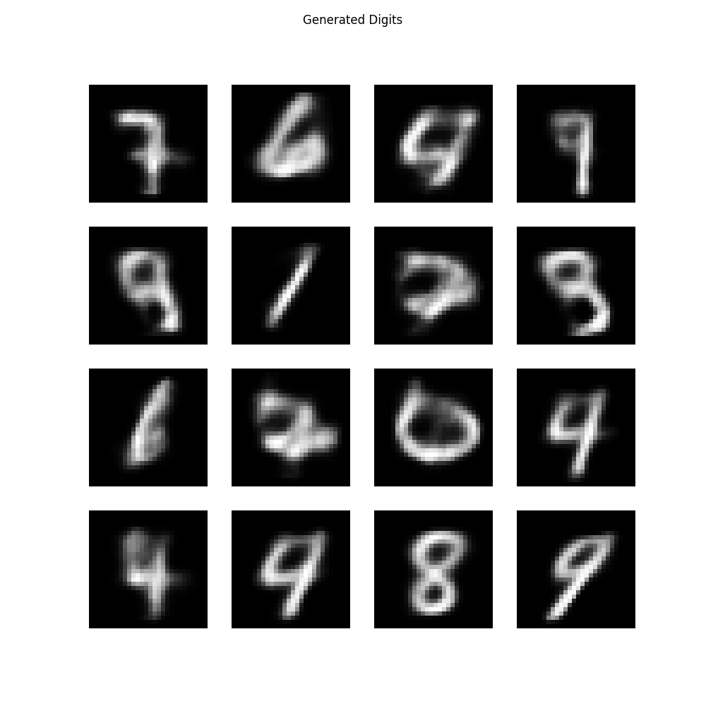
Also, the generated images from random samples look like digits, at least in most parts.

In image reconstruction we can use two different methods. We can choose to sample \(z\) or to use directly \(z=\mu\). Usually use cases prefer deterministic version for, well, more deterministic behaviour 😄

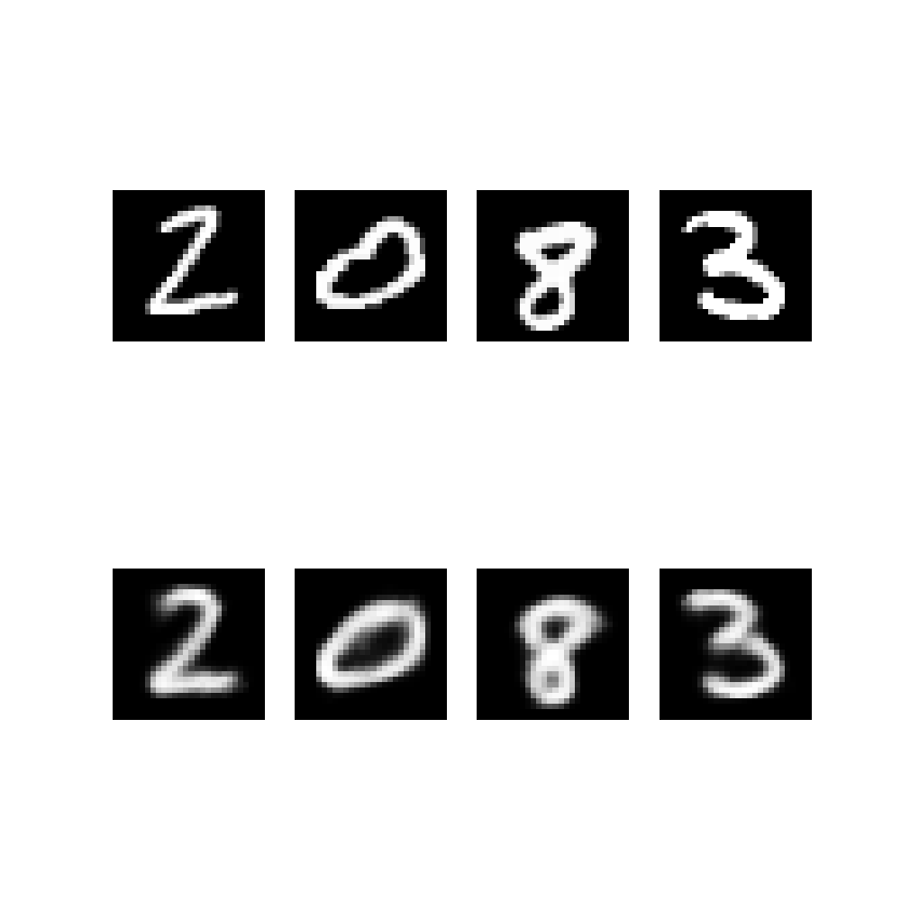
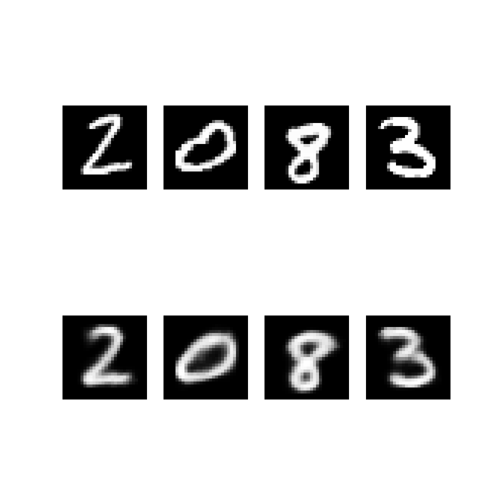
As we can notice, there is not much difference in this case.

Finally, lets try to travel in the latent space and visualize the journey. The 2d-mapping suggests to take the path 4 -> 7 -> 9.

It is not perfect, but for a few moments computing this is at least satisfactory.

Conclusion

The latent space is now clearly better behaving. We can demonstrate generative nature by traveling within it and decoding the images on the way.

There is a lot to discuss about the idea of latent spaces and I hope to have time to compile a post of the topic. I think Wittgenstein touched the idea in his writings about written language versus "what really exists".

The next article will be about diffusion models.