Dimension reductions: t-SNE

Jani Isohanni

04 Mar 2026 • 11 min read

T-SNEis well-known dimensionality reduction algorithm particularly suited for the visualization of high-dimensional datasets. This article goes through the mathematics behind t-SNE and provides a simple, pedagogical Python-implementation on the way.

T-SNE stands for t-Distributed Stochastic Neighbor Embedding and it is a non-linear method.

It is particularly good at preserving local structure in the data, meaning that points that are close together in high-dimensional space will also be close together in the low-dimensional representation.
It does not preserve global structure well, meaning that distances between clusters in the low-dimensional space may not accurately reflect their relationships in the high-dimensional space.
It is computationally intensive, especially for large datasets, and may require careful tuning of hyperparameters such as perplexity and learning rate.

We will go through the basic mathematical concepts of t-SNE and provide a simple demonstrative implementation with Python using numpy.

Preliminaries

Probability distribution

A probability distribution is a function that provides the probabilities of occurrence of different possible outcomes in an experiment.
Perhaps the most common probability distribution is the Gaussian (or normal) distribution, which is characterized by its bell-shaped curve. Its probability density function is defined as:\[f(x) = \frac{1}{\sigma \sqrt{2\pi}} e^{-\frac{(x-\mu)^2}{2\sigma^2}}\]
where \(\mu\) is the mean and \(\sigma\) is the standard deviation.

Another example of a probability distribution is the Student's t-distribution, which is often used when dealing with small sample sizes or when the population standard deviation is unknown. Its probability density function is defined as: \[f(x) = \frac{\Gamma\left(\frac{\nu + 1}{2}\right)}{\sqrt{\nu \pi} \Gamma\left(\frac{\nu}{2}\right)} \left(1 + \frac{x^2}{\nu}\right)^{-\frac{\nu+1}{2}}\]

where \(\nu\) is the degrees of freedom and \(\Gamma\) is the gamma function.

We will need both in our discussion of t-SNE.

Kullback-Leibler divergence

Kullback-Leibler (KL) divergence is a measure of how one probability distribution diverges from a second, expected probability distribution. It is defined as:
\[D_{KL}(P || Q) = \sum_{i} P(i) \log\left(\frac{P(i)}{Q(i)}\right)\]
where \(P\) and \(Q\) are the two probability distributions.

KL-divergence would certainly deserve a post of it own, but for now we limit to some basic characteristics of it.

KL-divergence is always non-negative, meaning that \(D_{KL}(P || Q) \geq 0\) for all probability distributions \(P\) and \(Q\).
KL-divergence is zero if and only if the two distributions are identical, i.e., \(D_{KL}(P || Q) = 0\) if \(P(i) = Q(i)\) for all \(i\).
KL-divergence is not symmetric, meaning that \(D_{KL}(P || Q) \neq D_{KL}(Q || P)\).

The intuition is that is measures how much information is lost when \(Q\) is used to approximate \(P\). As you can see, it is not a true distance metric since it does not satisfy the symmetry property. It is rooted in information theory and especially in Shannon's concept of entropy.

Gradient descent

Gradient descent is an optimization algorithm used to minimize a function by iteratively moving towards the steepest descent, which is the negative of the gradient. It is, in essence, a way to find the minimum of a function by taking small steps in the direction of the negative gradient (or derivative in high-school algebra terms).

The basic idea behind gradient descent is to start with an initial guess for the minimum and then update that guess iteratively by taking small steps in the direction of the negative gradient. The size of the steps is determined by a learning rate, which controls how big steps algorithm takes in the process.

The update rule for gradient descent can be expressed as:
\[\theta_{new} = \theta_{old} - \alpha \nabla f(\theta_{old})\]
where \(\theta\) represents the parameters being optimized, \(\alpha\) is the learning rate, and \(\nabla f(\theta_{old})\) is the gradient of the function at the current parameter values.

T-SNE algorithm

In dimension reduction we take a set of high-dimensional data points and map them to a lower-dimensional space while preserving certain properties of the original data. In t-SNE case, we usually map to 2D or 3D space for visualization purposes.
The elements in high-dimensional space are represented as \((x_1, x_2, \ldots, x_N)\) and their corresponding low-dimensional representations as \((y_1, y_2, \ldots, y_N)\). Our goal is to find the set of points \((y_i)\) that best represent
the original points \((x_i)\) in the lower-dimensional space, and in t-SNE the emphasis (i.e. the definition of "best") is on preserving local structure (meaning clusters).

The t-SNE algorithm consists of several steps:

Compute pairwise affinities in high-dimensional space: For each pair of points in the high-dimensional space, compute a similarity measure using a Gaussian distribution.
Compute pairwise affinities in low-dimensional space: Similarly, compute pairwise similarities in the low-dimensional space using a Student's t-distribution.
Minimize the KL-divergence: Use gradient descent to minimize the KL-divergence between the two distributions of similarities.

The overall process is rather simple, but the details of each step are slightly involved.

Step 1: Compute pairwise affinities in high-dimensional space

As mentioned, we start by computing the pairwise affinities between points in the high-dimensional space. This is done by manipulating the euclidean distances using probability distributions, namely Normal distribution in the high-dimensional space. What this means is that we interpreted the similarity between two points as the probability that one point would pick the other as its neighbor if neighbors were picked in proportion to their probability density under a Gaussian centered at the first point.

Now, in order to compute these probabilities, we first define a conditional probability \((p_{j|i})\) that point \((x_i)\) would pick point \((x_j)\) as its neighbor (this is sometimes called similarity of \(x_i\) and \(x_j\)):
\[p_{j|i} = \frac{\exp(-||x_i - x_j||^2 / 2\sigma_i^2)}{\sum_{k \neq i} \exp(-||x_i - x_k||^2 / 2\sigma_i^2)}\]
where \(\sigma_i\) is the bandwidth of the Gaussian kernel for point \(x_i\).
The bandwidth \(\sigma_i\) is chosen such that the perplexity of the distribution \(P_i\) matches a user-defined perplexity value.

Perplexity is defined as:
\[Perp(P_i) = 2^{H(P_i)}\]
where \(H(P_i)\) is the Shannon entropy of the distribution \(P_i\).

Now, we'll start by computing the Euclidean distances between all pairs of points in the high-dimensional space, and then we will convert these distances into probabilities using the Gaussian kernel.
The Euclidean distance between two points \(x_i\) and \(x_j\) is defined by:
\[d_{ij} = |x_i - x_j|^2\]
and we can manipulate it to
\[|x_i - x_j|^2 = (x_i - x_j)\cdot (x_i - x_j) = x_i\cdot x_i + x_j\cdot x_j - 2x_i\cdot x_j \] \[= |x_i|^2 + |x_j|^2 - 2x_i\cdot x_j\]
which provides a more efficient way to compute the distances using matrix operations.

In Python we can implement this step as follows:

    def _compute_squared_distances(self, X):
      """Compute squared distance in Euclidean metric"""
      n = X.shape[0]

      # sum_X[i] = x_i[0]² + x_i[1]² + ... + x_i[n-1]² = ||x_i||²
      sum_X = np.sum(X**2, axis=1)

      # sum_X.reshape(-1, 1) is n-by-1 column vector with elements ||x_i||², sum_X.reshape(1, -1) is 1-by-n vector with elements ||x_j||², 
      # so their sum gives us the ||x_i||^2 + ||x_j||^2 part for all pairs (i,j) and then we just subtract 2 * X @ X.T to get the full distance matrix.
      D = sum_X.reshape(-1, 1) + sum_X.reshape(1, -1) - 2 * X @ X.T

      # Some final stabilization steps.
      np.fill_diagonal(D, 0)
      return np.maximum(D, 0)

Next we need to find the appropriate value of \(\sigma_i\) for each point \(x_i\) such that the perplexity of the distribution \(P_i\) matches a user-defined perplexity value. We do this using binary search.
The overall construction is simple. We start with an initial guess for \(\sigma_i\) and compute the corresponding probabilities \(p_{j|i}\). We then compute the perplexity of this distribution and compare it to the desired perplexity.If the computed perplexity is too high, we need to increase \(\sigma_i\) to make the distribution more spread out. If the computed perplexity is too low, we need to decrease \(\sigma_i\) to make the distribution more concentrated.

We repeat this process until we find a value of \(\sigma_i\) that gives us the desired perplexity.

In Python this is simple

        P = np.zeros((n, n))
        for i in range(n):
            sigma_i = self._find_kernel_width(distances_sq[i], i, self.perplexity)
            P[i] = self._compute_conditional_affinities(distances_sq[i], i, sigma_i)

Where we first find the sigmas with binary search

    def _find_kernel_width(self, distances_sq_i, i, target_perplexity):

    sigma_min = 1e-20
    sigma_max = 1e20
    sigma = 1.0
    
    for _ in range(50):
        affinities_i = self._compute_conditional_affinities(distances_sq_i, i, sigma)
        H = self._compute_shannon_entropy(affinities_i)
        perplexity = 2 ** H
        
        if abs(perplexity - target_perplexity) < 1e-5:
            break
            
        if perplexity > target_perplexity:
            sigma_max = sigma
            sigma = (sigma + sigma_min) / 2
        else:
            sigma_min = sigma
            sigma = (sigma + sigma_max) / 2
    
    return sigma

Notice that Perplexity function is monotonic, which justifies the use of binary search and ensures its convergence. Next we compute the conditional affinities using the Gaussian kernel:

def _compute_conditional_affinities(self, distances_sq_i, i, sigma):
    # Gaussian kernel: exp(-||x_i - x_j||^2 / 2*sigma^2)
    affinities = np.exp(-distances_sq_i / (2 * sigma**2))
    affinities[i] = 0  
    affinities = affinities / (np.sum(affinities) + 1e-8)  # Normalize to get probabilities
    return affinities

Now we only need to symmetrize the affinities to get the final joint probabilities \(P_{ij}\):

P = (P + P.T) / 2

One needs to be careful here. In general we should not expect that \(P[i,j] = P[j,i]\) since they are computed independently and the space might look very different from different points, but we want to have a symmetric matrix of affinities. Hence we are taking the average of the two to ensure symmetry.

Secondly, when computing the affinities, we normalize per row, not per matrix, which means that the sum of each row of \(P\) is \(1\), but the sum of the entire matrix \(P\) is \(n\). For the KL-divergence we need
to normalize the entire matrix so that it sums to 1, which is done by dividing by n:

P = P / np.sum(P)

And we are done this part.

Step 2: Compute pairwise affinities in low-dimensional space

First we initialize the low-dimensional representations \(y_i\) randomly.

np.random.randn(n_samples, self.n_components) * 1e-4

Here the goal is to have the starting points close to the origo. This ensures that there is no predefined structure in the low-dimensional space that could bias the optimization process. Also the points "see each other" from the start, which is important for the optimization process to work well because it helps to avoid potential local minima or valleys in the optimization landscape.

Before entering the actual KL-divergence computation, we will exaggerate the affinities in high-dimensional space.

P_exaggerated = P * self.early_exaggeration

This is to provide better separation between clusters in the early stages of optimization, which can help to avoid local minima and improve the overall quality of the embedding. The value used here is typically around 4 or 12, and it is a hyperparameter that can be tuned based on the dataset and the desired visualization. There is no clear theoretical justification for the values used, they were found empirically over time.

Step 3: Minimize the KL-divergence

Now we are ready to compute the KL-divergence between the two distributions of similarities and use gradient descent to minimize it.

Y = self._optimize(P_exaggerated, P, Y)

The overall process is as follows. We first compute the affinities in the low-dimensional space using the Student's t-distribution. Then we compute the gradient of the KL-divergence with respect to the low-dimensional representations \(Y\) and update \(Y\) using gradient descent.

But here the implementation of the gradient descent is a bit more involved, as it includes momentum and adaptive learning rates, which are techniques used to improve the convergence of the optimization process.
These tricks are engineering details and they don't really carry any strong theoretical justification, but they are found to work well in practice.

The gradient descent is defined Y = Y - learning_rate * gradient.

We will use a momentum gradient descent, which means that we will keep track of the previous update and use it to influence the current update. This helps to accelerate convergence and avoid local minima.

velocity = momentum * velocity - learning_rate * gradient

Y = Y + velocity

This trick accelerates the convergence of the optimization process by allowing the algorithm to "remember" the previous updates and use them to influence the current update. Altough the momentum is less than one, the overall
cumulative effect of the previous updates can be significant, especially when the gradients are consistent over multiple iterations. Further, this helps to smooth out the optimization trajectory and avoid oscillations or getting stuck in local minima.

Assume a constant gradient g over multiple iterations. The cumulative effect of the momentum term can be expressed as:
\[ g \cdot \left( \frac{\alpha}{1 - \beta} \right)\]
where \(\alpha\) is the learning rate and \(\beta\) is the momentum coefficient.
This shows that even with a momentum coefficient less than one, the cumulative effect of the previous updates can be significant, especially when the gradients are consistent over multiple iterations.

In t-SNE we will use t-distribution with one degree of freedom (which is equivalent to the Cauchy distribution) to compute the affinities in the low-dimensional space. The point density funtion of the t-distribution is then defined as:
\[\frac{1}{\pi(1 + t^2)}\]

This translates to the following code (notice that \(\pi\) cancels out):

 def _compute_low_dim_affinities(self, Y):
    sum_Y = np.sum(Y**2, axis=1)
    distances_sq = sum_Y.reshape(-1, 1) + sum_Y.reshape(1, -1) - 2 * Y @ Y.T
    
    # Student's t-kernel: (1 + ||y_i - y_j||^2)^-1
    Q = 1 / (1 + distances_sq)
    np.fill_diagonal(Q, 0)
    
    # Normalize
    Q = Q / np.sum(Q)
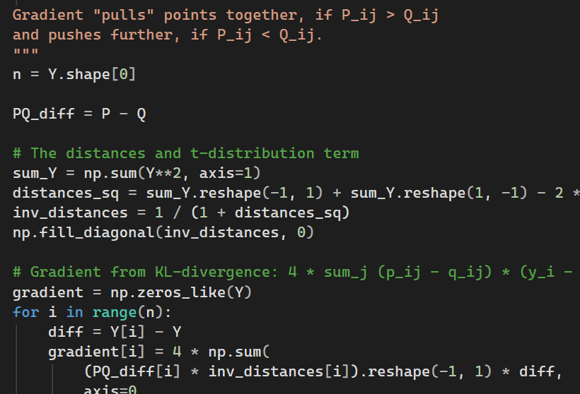
    Q = np.maximum(Q, 1e-12)

Now we need to compute the gradient based on the KL-divergence between the two distributions \(P\) and \(Q\). The gradient is rather straightforward to derive, and we get
\[4 \sum_j (p_{ij} - q_{ij}) * (y_i - y_j) * (1 + d_{ij}^2)^{-1}.\]

We only need to compute it

def _compute_gradient(self, P, Q, Y):
    n = Y.shape[0]
    PQ_diff = P - Q
    
    sum_Y = np.sum(Y**2, axis=1)
    distances_sq = sum_Y.reshape(-1, 1) + sum_Y.reshape(1, -1) - 2 * Y @ Y.T
    inv_distances = 1 / (1 + distances_sq)
    np.fill_diagonal(inv_distances, 0)
    
    # Gradient from KL-divergence: 4 * sum_j (p_ij - q_ij) * (y_i - y_j) * (1 + d_ij^2)^-1
    gradient = np.zeros_like(Y)
    for i in range(n):
        diff = Y[i] - Y
        gradient[i] = 4 * np.sum(
            (PQ_diff[i] * inv_distances[i]).reshape(-1, 1) * diff,
            axis=0
        )

You need to be careful with the dimensions, but otherwise this is a routine implementation.

Now the full computation still carries some tricks. As you noticed, we used P_exaggerated in the process. This is to boost the attractive forces in the early stages of optimization, which speeds up the convergence and helps to create better separation between clusters. We will drop the exaggeration after a certain number of iterations (another hyperparameter).

Further, we will also use aforementioned momentum and adaptive learning rate to improve the convergence. Again, these are engineering details that don't have a strong theoretical justification, but they are found to work well in practice.

The full process would hence be as follows.

        momentum = 0.5
        final_momentum = 0.8
        momentum_switch_iter = 250
        
        Y_delta = np.zeros_like(Y)
        
        for iteration in range(self.n_iter):

            P_current = P_exaggerated if iteration < self.early_exaggeration_iter else P
            
            if iteration == momentum_switch_iter:
                momentum = final_momentum
            
            Q = self._compute_low_dim_affinities(Y)
            gradient = self._compute_gradient(P_current, Q, Y)
            
            Y_delta = momentum * Y_delta - self.learning_rate * gradient
            Y = Y + Y_delta
            
            Y = Y - np.mean(Y, axis=0)
            
            if (iteration + 1) % 100 == 0:
                kl_div = self._compute_kl_divergence(P_current, Q)
                print(f"Iteration {iteration + 1}: KL divergence = {kl_div:.4f}")
             ```

This implementation is far from optimal and it is dead slow, but it serves the purpose of demonstrating the core ideas behind t-SNE.

One question one would think here is why t-distribution? The folklore is that it was found to work well empirically. Engineering, yet again. But there is more to it.

The t-distribution has heavier tails than the Gaussian distribution, which means that it can better capture the local structure of the data in the low-dimensional space. Consider points A, B and C in the high-dimensional space, where A and B are close to each other, and C is far from both A and B.
In the low-dimensional space, we want to preserve the local structure, which means that A and B should be close together, while C should be farther away.
Now that we have t-distribution with heavier tails, it does allow the local clusters to push each other apart more effectively.
That, in turn, helps to prevent the crowding problem and allows for a more faithful representation of the local structure in the low-dimensional space.

When using t-SNE, you should acknowledge that it does not map the data to a low-dimensional space in a way that preserves global structure. It does not map data at all.
It creates a new representation of the data in a low-dimensional space that emphasizes local structure. And this is the core reason (with the fact that KL-divergense is not symmetric) it does not invert.

This dynamics can be seen in the gradient of the KL-divergence, which consists of two terms. Attractive term that pulls points together based on the high-dimensional affinities \(P_{ij}\),
and a repulsive term that pushes points apart based on the low-dimensional affinities \(Q_{ij}\).

\[\frac{\partial C}{\partial y_i} \propto \sum_j (p_{ij} - q_{ij}) \cdot (y_i - y_j) \cdot \left[1 + |y_i - y_j|^2\right]^{-1}\]

T-distribution's heavier tails ensure that the repulsive forces do not vanish too quickly as points move apart. This prevents points from collapsing into a single cluster in the low-dimensional space.