Autoencoders: The Foundation of Generative AI

The world of deep learning has evolved dramatically over the last decade or two. While on my post-graduate studies around 2010, the neural networks were mostly a mathematical model that was way too expensive to train for many practical tasks. Todays hardware evolution and the innovations in network architectures have changed that totally.

These changes motivated me to explore the world a bit more deeply. I wanted to understand how generative AI actually works, and I do not mean large language models but those that turn textual presentations to images or even videos. Personally that really feels like magic even (or perhaps because of..?) that I happen to have strong mathematical background and know how the networks works conceptually.

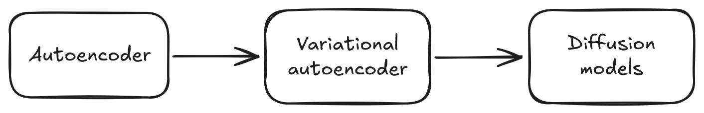
Anyway, after browsing the subject a bit it came clear I need to start this journey from autoencoders. It seems the evolution has been from autoencoders to variational autoencoders and finally to the state-of-the-art architectures with diffusion models. So this is the path I chose, and I decided to document my learnings in case someone prefers reading technical content over watching videos.

You can find the code from my GitHub repository.

Autoencoder Concept

In traditional (I mean ancient, like around 2010) machine learning algorithms it was up to human to extract and code the information of the subject(s) and object(s) in hand. Humans have already intellectually processed things to words and descriptions, meaning that "things" have "names" (more philosophically oriented might recognize the relation to the works of Wittgenstein).

This understanding was then hand-coded to the algorithm. For example, a license plate was extracted, translated, perhaps denoised and otherwise processed, and then, finally, the actual ML did the magic (in this context it was basically OCR). This is feature-engineering, i.e. extracting the features of interest by hand from the data.

This preprocessing was hand-made for several reasons.

Usually the amount of training data was not that big which means that the more we could manually guide the system towards the right direction, the more efficiently we can use the material to train the real core issue. There is no point to "waste" training material to teach the neural network (or whatever the architecture was) to spot a license plate when can do that with some manual effort.

Another reason was simply that the computing capacity was not there, and this has changed quite a lot. Further, the understanding of the neural network architectures was very limited and it was not that easy to know what to apply in each case. This also has evolved drastically.

Now, what if you could teach neural network to spot the features automatically? You would drop the feature engineering step altogether and the network could form an understanding from the data with no guidance, whatsoever. Sounds like general intelligence, does it?

If you think of this problem, how would you even start to solve it?

The features are usually intuitive hence natural to human but not to computers. You can describe the feature space to a colleague, but how to make computer to understand it? Textual presentation hardly turns to a visual categorization method for computers.

It turns out you actually can do this. You can train a model to automatically learn a feature in a self-supervised manner.

First, consider what a feature is.

I would describe it as the foundational information we have of the class of the objects in hand. It can be "these figures have numbers" or "there is a dog in this image". A feature encapsulates something very inherent of the data. And when you manage to encapsulate enough of these very inherent features, what you can do with that information?

You can reconstruct the object.

If we know we have "number 1", "hand drawn", "blue foreground" and "white background" with some technical details like resolution and color space, we can reconstruct a representation of the object, and sure enough the reconstruction would carry these features.

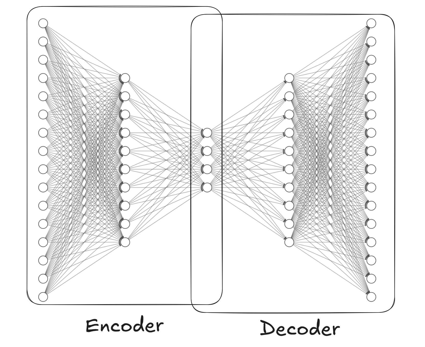
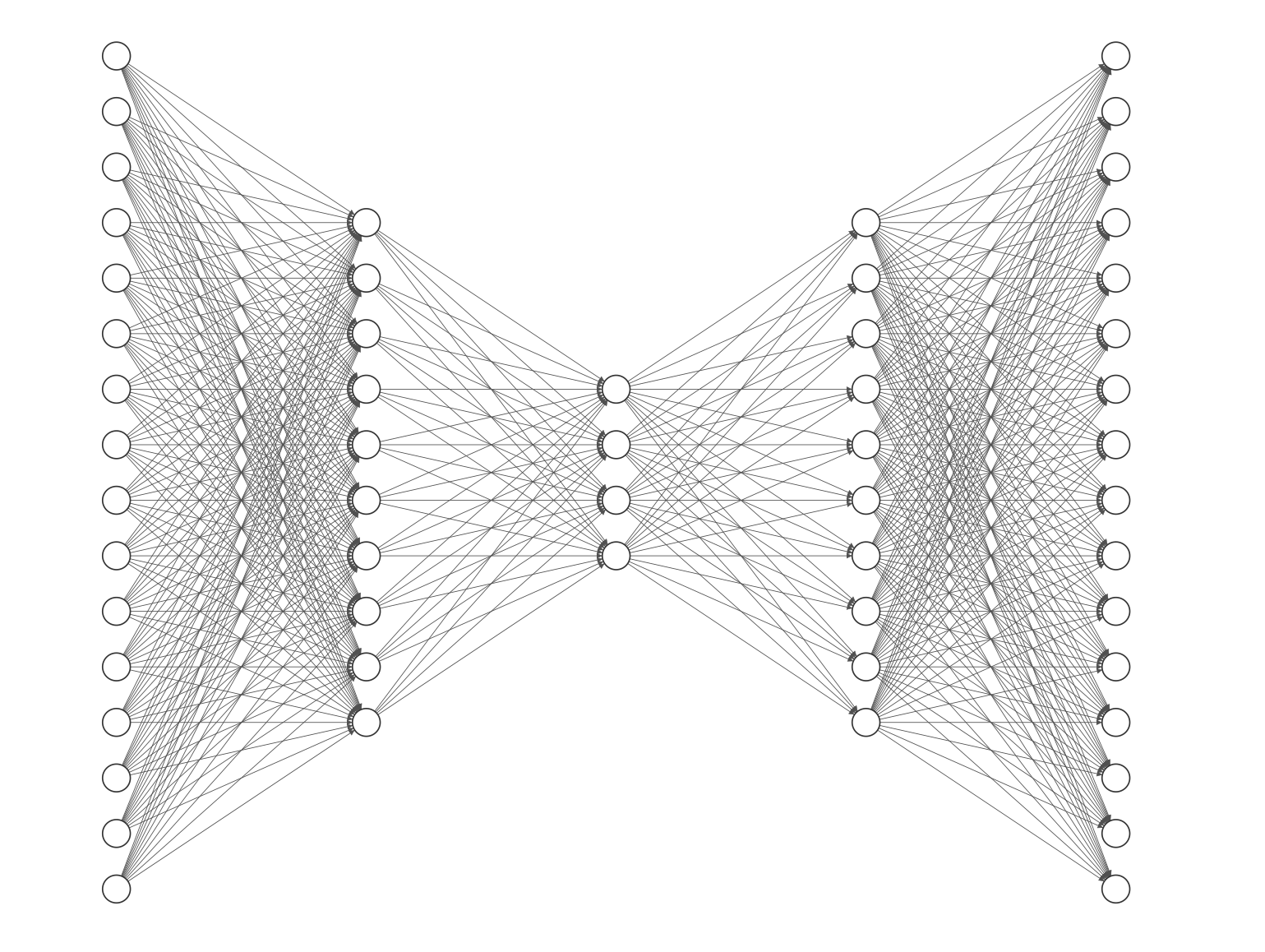
This observation leads us to the very core structure of autoencoders. In autoencoders we separate encoder and decoder. First, the encoder is a network that squeezes the original data into a lower dimension space "latent space". Then decoder uses this low-dimensional representation to reconstruct the original image. And we train the model by computing loss of the constructed object from the original one.

Because we force the network to "compress" (encode) the original image to a lower dimensional space by requiring it to be able to reconstruct (decode) it, we actually force it to extract the best features for the process.

Notice that in this case a "feature" is not an intuitive feature like "dog", but a mathematical reduction of the data that preserves the most important aspects of it. The network in a way forms its own succinct description of the data. When you train the network with data that has some shared patterns, the internal layer learns to extract those patterns.

Autoencoder in Denoising

Technically autoencoders are dead simple. You create encoder and decoder, train the model and... well, off you go with your use case.

There are various use cases for AEs. Anomaly detection, denoising, compression, dimension reduction etc. But in generative AI autoencoders are not that widely used and they are currently superseded more sophisticated models and methods.

To demonstrate how they work we use MNIST-dataset that has hand drawn digits. It is perhaps the most widely used dataset and it happens to visualize the characteristics of AEs quite nice.

We could go with just reconstruction to see how the network learns the features of the images, but let us take a step further and use the network for denoising. This makes the point even more compelling; even if we train the model with noisy images, it can distinguish digits and hence form separate clusters in the latent space.

First we create a simple autoencoder model.

class Autoencoder(nn.Module):
    def __init__(self, latent_dim=32):
        super().__init__()
        # Encoder
        self.fc1 = nn.Linear(784, 400)
        self.fc2 = nn.Linear(400, latent_dim)
        
        # Decoder
        self.fc3 = nn.Linear(latent_dim, 400)
        self.fc4 = nn.Linear(400, 784)
    
    def encode(self, x):
        h = F.relu(self.fc1(x))
        return self.fc2(h)
    
    def decode(self, z):
        h = F.relu(self.fc3(z))
        return torch.sigmoid(self.fc4(h))
    
    def forward(self, x):
        z = self.encode(x.view(-1, 784))
        return self.decode(z)
        ```

Then we train it.

Let us try this for denoising and add some noise to the input image and compute the loss against the image without noise.

The dataset is very simple and we seem to reach satisfactory results with the following hyperparameter set. Play around with different values to get a feeling how they affect the results.

# Hyperparameters
latent_dim = 10  
batch_size = 128
epochs = 15
learning_rate = 1e-3
noise_factor = 0.3

In training we separate the training set from the test set. In this case the separation is already handled in the dataset, which makes our life easier.

# Data
transform = transforms.Compose([transforms.ToTensor()])
train_data = datasets.MNIST('./data', train=True, download=True, transform=transform)
train_loader = DataLoader(train_data, batch_size=batch_size, shuffle=True)
test_data = datasets.MNIST('./data', train=False, download=True, transform=transform)
test_loader = DataLoader(test_data, batch_size=batch_size, shuffle=False)

# Train the model
model = Autoencoder(latent_dim=latent_dim)
optimizer = torch.optim.Adam(model.parameters(), lr=learning_rate)

model.train()
for epoch in range(epochs):
    train_loss = 0
    for batch_idx, (data, _) in enumerate(train_loader):
        # Add noise to input
        noisy_data = add_noise(data, noise_factor)
        
        optimizer.zero_grad()
        recon_batch = model(noisy_data)
        # Loss: compare reconstruction to CLEAN data
        loss = F.mse_loss(recon_batch, data.view(-1, 784), reduction='sum')
        loss.backward()
        train_loss += loss.item()
        optimizer.step()
        ```

Denoising results

Let us first study the latent space. Now that we have a dataset with 10 different classes of images, one would expect the latent space to form clear clusters around these classes, right?

As the space is 10-dimensional, we can use UMAP to reduce it to 2D.

with torch.no_grad():
    z_list, labels_list = [], []
    for data, labels in test_loader:
        z = model.encode(data.view(-1, 784))
        z_list.append(z)
        labels_list.append(labels)
    
    z = torch.cat(z_list).numpy()
    labels = torch.cat(labels_list).numpy()
    
    plt.figure(figsize=(10, 8))
    
    reducer = umap.UMAP(random_state=42)
    z_2d = reducer.fit_transform(z)
    
    scatter = plt.scatter(z_2d[:, 0], z_2d[:, 1], c=labels, cmap='tab10', alpha=0.5, s=1)
    plt.colorbar(scatter)
    plt.tight_layout()
    plt.show()
    ```

The results are clear, the bottleneck forces the network to separate the numbers into different clusters just as expected.

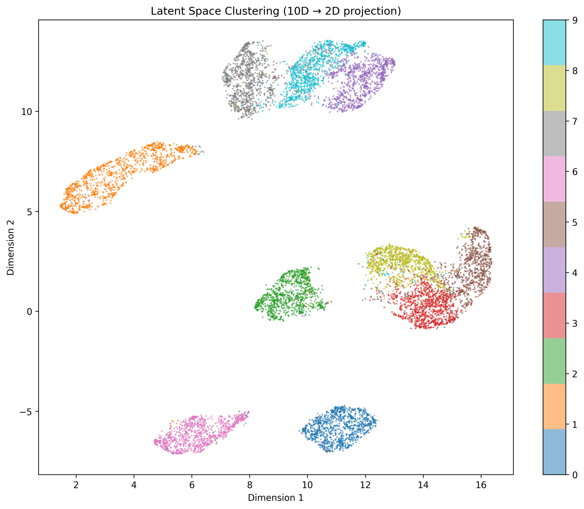
Clearly the model thinks 3, 5 and 8 are somewhat similar whereas 2, 6, 1 and 0 clearly form distant and separate clusters from others. Personally I find this result intuitive given the geometric nature of the digits.

Ok then, but how about reconstruction? Let us first compare the reconstruction capability without noise.

with torch.no_grad():
    data, _ = next(iter(test_loader))
    recon = model(data[:8])
    
    fig, axes = plt.subplots(2, 8, figsize=(12, 3))
    for i in range(8):
        axes[0, i].imshow(data[i].squeeze(), cmap='gray')
        axes[0, i].axis('off')
        axes[1, i].imshow(recon[i].view(28, 28), cmap='gray')
        axes[1, i].axis('off')
    plt.tight_layout()
    plt.show()
    ```

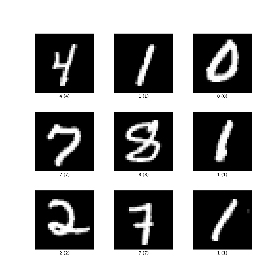
The result is good.

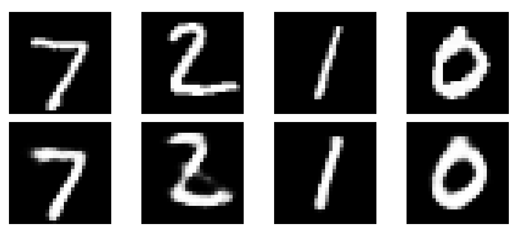
The reconstructed image clearly resembles the original one with some deviations. Notice that though the model was trained with images with noise, the reconstruction of clean images works quite well.

How about the final goal - denoising?

model.eval()
with torch.no_grad():
    data, _ = next(iter(test_loader))
    data = data[:8]
    noisy_data = add_noise(data, noise_factor)
    recon = model(noisy_data)
    
    fig, axes = plt.subplots(3, 8, figsize=(12, 5))
    for i in range(8):
        # Original
        axes[0, i].imshow(data[i].squeeze(), cmap='gray')
        axes[0, i].axis('off')
        # Noisy
        axes[1, i].imshow(noisy_data[i].squeeze(), cmap='gray')
        axes[1, i].axis('off')
        # Denoised
        axes[2, i].imshow(recon[i].view(28, 28), cmap='gray')
        axes[2, i].axis('off')
    
    plt.tight_layout()
    plt.show()
    ```

It turns out to work quite well, indeed.

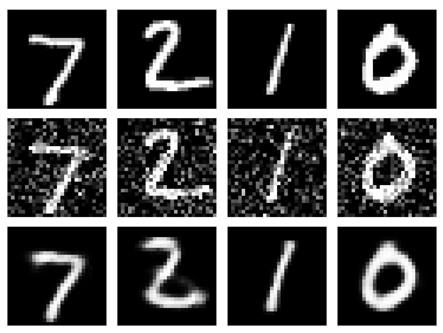
The denoised image is not perfect, but how the noise vanished is almost staggering especially given the extremely light architecture and training. Of course in this case the data is very simple and easy to learn, but even then the network performs quite well.

Conclusions

Autoencoders are, as mentioned, dead simple in their architecture. When thinking about generative AI, it would be tempting to use the latent space to generate images, right?

Problem is that the latent space is actually clustered in small areas which means that the actual subspace that could generate any meaningful image, is very small. If you try to generate images from random samples, you get nonsense.

with torch.no_grad():
    # Generate 6 random latent vectors
    random_z = torch.randn(6, latent_dim)
    generated = model.decode(random_z)
    
    fig, axes = plt.subplots(2, 3, figsize=(6, 4))
    for i in range(6):
        row = i // 3
        col = i % 3
        axes[row, col].imshow(generated[i].view(28, 28), cmap='gray')
        axes[row, col].axis('off')
    
    plt.suptitle('Random Samples from Decoder')
    plt.tight_layout()
    plt.savefig('random_generation.png', dpi=300, bbox_inches='tight')
    plt.show()
    ```

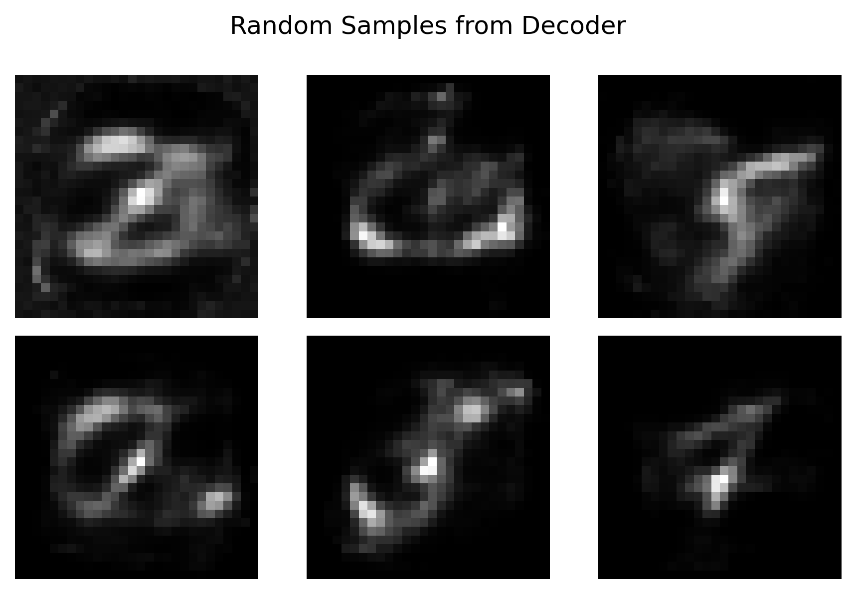
But there is a way to make the latent space more continuous, and that can provide more meaningful way to generate random numbers with the decoder. We will study that in the next article.